Bellhop - Ocean simulation modeling
What is BELLHOP ?
- BELLHOP is a beam tracing model for predicting acoustic pressure fields in ocean environments.
- BELLHOP can produce a variety of useful outputs including transmission loss, eigenrays, arrivals, and received time-series. It also allows for range-dependence in the top and bottom boundaries (altimetry and bathymetry), as well as in the sound speed profile (SSP).
- BELLHOP is implemented in Fortran, Matlab, and Python and used on multiple platforms (Mac, Windows, and Linux).

Figure 1: BELLHOP structure
WHY BELLHOP?
- Underwater communication channel is a relatively difficult transmission medium due to the variability of link quality depending on location and applications.
- Before deploying any kind of vehicles underwater, one should predict the underwater communication system performance which is based on the sound frequency transmitted underwater.
Why do you need to analyze the uw-comms performance?
-
To analyze impact of channel characteristics on underwater communications,
-
prior to deploying robots, predict communication system performance,
-
provide guidance on best physical layout to deploy underwater vehicles,
-
provide estimates on parameters for link budget calculation,
-
Because it will provide you a rough idea about how far you can communicate within network which is also known as an operation range for communication.
-
BELLHOP reads these files depending on options selected within the main environmental file.
-
There are various options for which you can run bellhop are:
- ray tracing option,
- eigenray option,
- transmission loss option,
- an arrivals calculation option.
🔧 Installation
📥 Download
- Latest Source Code (2024_12_25) (For Mac/Linux/Windows – must be built)
- Windows 10 Binary (2020_11_4) (older, includes MATLAB I/O)
💡 Note: Always check compile dates. Windows binaries are slower; building from source on your native architecture is recommended.
- If you’re using the Unix base system then open command prompt and go to the same folder where you extracted your zip.
cd at/at
make all
sudo make install
- If you’re using bellhop on Windows 10 machine then you also need to download the Win10 Binary executable files from here. Please also extract that to the folder at.
If something fails, run make clean and retry.
⚠️ Edit
Makefilefor proper architecture, Example for Linux-based machines:
export FFLAGS= -march=native -Bstatic -Waliasing -Wampersand -Wintrinsics-std -Wno-tabs -Wintrinsic-shadow -Wline-truncation -std=gnu -O1 -ffast-math -funroll-all-loops -fomit-frame-pointer -mtune=native
More help: Issue #3 on GitHub
Detailed Installation Instructions based on OS
📏 Bellhop 2D (Classic)
Bellhop computes underwater acoustic propagation using Gaussian beam tracing in a 2D vertical slice (range-depth). It is ideal for scenarios assuming cylindrical symmetry.
Sample Input Structure Explanation
Below is an annotated breakdown of a typical *.ENV input file for 2D Bellhop:
'arlpy'                             / Graph Title - just for Fortran/MATLAB
25000.000000                        / FREQUENCY
1                                   / [UNUSED]
'SVWT*'                             / (SSP INTERP METHOD)(TOP LAYER)(BOTTOM ATTENUATION UNITS)(VOLUME ATTENUATION)
1 0.0 100.000000                    / [UNUSED] [UNUSED] [MAX DEPTH]

0.000000   1540.400000              / [DEPTH] [SOUND SPEED]
10.000000  1540.500000              / [DEPTH] [SOUND SPEED]
20.000000  1540.700000              / [DEPTH] [SOUND SPEED]
30.000000  1534.400000              / [DEPTH] [SOUND SPEED]
50.000000  1523.300000              / [DEPTH] [SOUND SPEED]
75.000000  1519.600000              / [DEPTH] [SOUND SPEED]
100.000000 1518.500000              / [DEPTH] [SOUND SPEED]

'A' 0.000000                        / (BOTTOM LAYER)(EXTERNAL BATHYMETRY) [SIGMA BOTTOM ROUGHNESS]
100.000000 1600.000000 0.0 1.200000 1.000000 / [MAX DEPTH] [BOTTOM SOUND SPEED] [UNUSED] [DENSITY BOTTOM] [ATTENUATION BOTTOM]

1                                   / [NUMBER SOURCES]
50.000000                            / [SOURCE DEPTHS 1:N (m)]

1                                   / [NUMBER RECEIVER DEPTHS]
8.000000                             / [RECEIVER DEPTHS 1:N (m)]

1                                   / [NUMBER RECEIVER RANGES]
2.000000                             / [RECEIVER RANGES 1:N (km)]

'R *'                               / (RUN TYPE)(BEAM TYPE)(EXTERNAL SOURCE BEAM PATTERN) ; typically 'R', 'C', 'I', 'S'

0                                   / [NUMBER OF BEAMS]; 0 means bellhop auto-calculates
-80.000000 80.000000                / [MIN ANGLE] [MAX ANGLE]

0.0 101.000000 2.020000             / [STEP SIZE] [DEPTH BOX] [RANGE BOX]; 0 = default step size
Explanation of Bellhop 2D Parameters
TITLE: Descriptive label.FREQ: Acoustic frequency in Hz.NMEDIA: Usually set to 1 for a single ocean medium.SSPOPT: Interpolation method for SSP (e.g., ‘SVN’).DEPTH,SSP: Depth/sound speed pairs.NSD,SD: Number and values of source depths.NRD,RD: Number and values of receiver depths.NRR,RR: Number and values of receiver ranges.OPTION: Run type (e.g., ‘R’ for rays, ‘C’ for coherent TL).NBEAMS: Number of beams (or 0 for auto).ALPHA: Launch angles in degrees.STEP,ZBOX,RBOX: Step size and simulation domain bounds.
Bellhop 2D is particularly suitable for quick channel performance estimation and visualizing ray paths and arrival structures in a vertically stratified ocean.
For visual tools like plotray, plotshd, and plotarr, use output files .RAY, .SHD, and .ARR respectively.
📊 Visualizing with ARLPY
Sound Speed Profile
")
Figure 2: Sound Speed Profile of Bedford Basin (taken on 13-10-17)
How to Plot SSP’s using ARLPY ?
# SSP Plotting using ARLPY

import arlpy.uwapm as pm
import arlpy.plot as plt
import numpy as np

env = pm.create_env2d()
ssp = [
    [ 0, 1540],  # 1540 m/s at the surface
    [10, 1530],  # 1530 m/s at 10 m depth
    [20, 1532],  # 1532 m/s at 20 m depth
    [25, 1533],  # 1533 m/s at 25 m depth
    [30, 1535]   # 1535 m/s at the seabed
]
env = pm.create_env2d(soundspeed=ssp)
pm.plot_ssp(env, width=500)
Plotting an Environment
# Plotting an Environment using ARLPY

pm.plot_env(env, width=900)
Eigenrays
- Eigenray plots show just the rays that connect the source to a receiver.
# Eigenrays using ARLPY
import arlpy.uwapm as pm
import arlpy.plot as plt
import numpy as np

env = pm.create_env2d()
rays = pm.compute_eigenrays(env)
pm.plot_rays(rays, env=env, width=900)

Figure 3: Eigenrays using ARLPY
- compute the arrival structure at the receiver
arrivals = pm.compute_arrivals(env)
pm.plot_arrivals(arrivals, width=900)
arrivals[arrivals.arrival_number < 10][['time_of_arrival', 'angle_of_arrival', 'surface_bounces', 'bottom_bounces']]
| time_of_arrival | angle_of_arrival | surface_bounces | bottom_bounces | |
|---|---|---|---|---|
| 1 | 0.721796 | 22.538254 | 9 | 8 |
| 2 | 0.716791 | -21.553932 | 8 | 8 |
| 3 | 0.709687 | 20.052078 | 8 | 7 |
| 4 | 0.705226 | -19.034414 | 7 | 7 |
| 5 | 0.698960 | 17.484421 | 7 | 6 |
| 6 | 0.695070 | -16.436060 | 6 | 6 |
| 7 | 0.689678 | 14.842224 | 6 | 5 |
| 8 | 0.686383 | -13.766296 | 5 | 5 |
| 9 | 0.681901 | 12.133879 | 5 | 4 |
| 10 | 0.679223 | -11.034208 | 4 | 4 |
# convert to a impulse response time series

ir = pm.arrivals_to_impulse_response(arrivals, fs=96000)
plt.plot(np.abs(ir), fs=96000, width=900)
Bathymetry
Let’s first start off by defining our bathymetry, a steep up-slope for the first 300 m, and then a gentle downslope:
# add/change bathy to env
bathy = [
    [0, 30],    # 30 m water depth at the transmitter
    [300, 20],  # 20 m water depth 300 m away
    [1000, 25]  # 25 m water depth at 1 km
]

# add/change SSP to env
ssp = [
    [ 0, 1540],  # 1540 m/s at the surface
    [10, 1530],  # 1530 m/s at 10 m depth
    [20, 1532],  # 1532 m/s at 20 m depth
    [25, 1533],  # 1533 m/s at 25 m depth
    [30, 1535]   # 1535 m/s at the seabed
]

# Appending ssp and bathy to existing env file
env = pm.create_env2d(
    depth=bathy,
    soundspeed=ssp,
    bottom_soundspeed=1450,
    bottom_density=1200,
    bottom_absorption=1.0,
    tx_depth=15
)
pm.print_env(env)


                    name : arlpy
       bottom_absorption : 1.0
          bottom_density : 1200
        bottom_roughness : 0
       bottom_soundspeed : 1450
                   depth : [[   0.   30.]
                            [ 300.   20.]
                            [1000.   25.]]
            depth_interp : linear
               frequency : 25000
               max_angle : 80
               min_angle : -80
                  nbeams : 0
                rx_depth : 10
                rx_range : 1000
              soundspeed : [[   0. 1540.]
                            [  10. 1530.]
                            [  20. 1532.]
                            [  25. 1533.]
                            [  30. 1535.]]
       soundspeed_interp : spline
                 surface : None
          surface_interp : linear
                tx_depth : 15
       tx_directionality : None
                    type : 2D


pm.plot_env(env, width=900)
Looks more interesting! Let’s see what the eigenrays look like, and also the arrival structure:
rays = pm.compute_eigenrays(env)
pm.plot_rays(rays, env=env, width=900)
We could also ignore the receiver, and plot rays launched at various angles:
rays = pm.compute_rays(env)
pm.plot_rays(rays, env=env, width=900)
import numpy as np
from scipy.interpolate import griddata
import scipy.ndimage as ndimage
from scipy.ndimage import gaussian_filter
import scipy
# from scipy.misc import imsave
from matplotlib import cm
import matplotlib.pyplot as plt
from mpl_toolkits.mplot3d import Axes3D
from stl import mesh, Mode
import matplotlib.tri as mtri
from mpl_toolkits.mplot3d.axes3d import get_test_data
from pandas import read_csv


data = read_csv('bathy.txt', sep='\s+', header=None, names=['x', 'y', 'depth'])

x = np.arange(data.x.min(), data.x.max()+1)
y = np.arange(data.y.min(), data.y.max()+1)

X, Y = np.meshgrid(x, y)

Z = griddata(data[['x','y']].values, -data['depth'].values, (X, Y), method='linear')

# make the grid square
Z[np.isnan(Z)] = 0

fig = plt.figure(figsize=(14, 8))
ax = fig.add_subplot(111)
plt.imshow(Z)
plt.show()
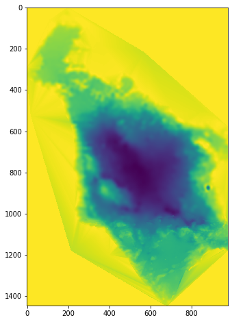
Figure 4: Bedford Basin Bathy 2D

Figure 5: Bedford Basin Bathy 3D
or place lots of receivers in a grid to visualize the acoustic pressure field (or equivalently transmission loss). We can modify the environment (env) without having to recreate it, as it is simply a Python dictionary object:
env['rx_range'] = np.linspace(0, 1000, 1001)
env['rx_depth'] = np.linspace(0, 30, 301)
Transmission Loss
- The number of beams, NBeams, should normally be set to 0, allowing BELLHOP to automatically select the appropriate value. The number needed increases with frequency and the maximum range to a receiver.
- RUN TYPE BELLHOP

OPTION(1:1):           'R' generates a ray file
                       'E' generates an eigenray file
                       'A' generates an amplitude-delay file (ascii)
                       'a' generate  an amplitude-delay file (binary)
                       'C' Coherent     TL calculation
                       'I' Incoherent   TL calculation
                       'S' Semicoherent TL calculation
                            (Lloyd mirror source pattern)
- The pressure field, p, is then calculated for the specified grid of receivers, with a scaling such that $20\ log10(|p|)$ is the transmission loss in dB.
tloss = pm.compute_transmission_loss(env)
pm.plot_transmission_loss(tloss, env=env, clim=[-60,-30], width=900)
We see a complicated interference pattern, but an interesting focusing at 800 m at a 15 m depth. The detailed interference pattern is of course sensitive to small changes in the environment. A less sensitive, but more averaged out, transmission loss estimate can be obtained using the incoherent mode:
tloss = pm.compute_transmission_loss(env, mode='incoherent')
pm.plot_transmission_loss(tloss, env=env, clim=[-60,-30], width=900)
Source directionality
- Now, let’s use a directional transmitter instead of an omni-directional one:
beampattern = np.array([
    [-180,  10], [-170, -10], [-160,   0], [-150, -20], [-140, -10], [-130, -30],
    [-120, -20], [-110, -40], [-100, -30], [-90 , -50], [-80 , -30], [-70 , -40],
    [-60 , -20], [-50 , -30], [-40 , -10], [-30 , -20], [-20 ,   0], [-10 , -10],
    [  0 ,  10], [ 10 , -10], [ 20 ,   0], [ 30 , -20], [ 40 , -10], [ 50 , -30],
    [ 60 , -20], [ 70 , -40], [ 80 , -30], [ 90 , -50], [100 , -30], [110 , -40],
    [120 , -20], [130 , -30], [140 , -10], [150 , -20], [160 ,   0], [170 , -10],
    [180 ,  10]
])
env['tx_directionality'] = beampattern
tloss = pm.compute_transmission_loss(env)
pm.plot_transmission_loss(tloss, env=env, clim=[-60,-30], width=900)
- Now you can see the directionality and the sidelobe structure of the transmitter.
tloss = pm.compute_transmission_loss(env, mode='incoherent')
pm.plot_transmission_loss(tloss, env=env, clim=[-60,-30], width=900)
Undulating water surface
- Finally, let’s try adding a long wavelength swell on the water surface:
surface = np.array([[r, 0.5+0.5*np.sin(2*np.pi*0.005*r)] for r in np.linspace(0,1000,1001)])
env['surface'] = surface
tloss = pm.compute_transmission_loss(env)
pm.plot_transmission_loss(tloss, env=env, clim=[-60,-30], width=900)
tloss = pm.compute_transmission_loss(env, mode='incoherent')
pm.plot_transmission_loss(tloss, env=env, clim=[-60,-30], width=900)
- Now, if I placed a receiver at 800 m, and 15 m depth, roughly where we see some focusing, what would the eigenrays and arrival structure look like?
env['rx_range'] = 800
env['rx_depth'] = 15

rays = pm.compute_eigenrays(env)
pm.plot_rays(rays, env=env, width=900)
arrivals = pm.compute_arrivals(env)
pm.plot_arrivals(arrivals, dB=True, width=900)
Note: We plotted the amplitudes in dB, as the later arrivals are much weaker than the first one, and better visualized in a logarithmic scale.
Bellhop3D – 3D Beam Tracing for Complex Ocean Environments
-
BELLHOP3D is a beam tracing model for predicting acoustic pressure fields in ocean environments.
-
It is an extension to 3D environments of the popular BELLHOP model and includes (optionally) horizontal refraction in the lat-long plane.
-
3D pressure fields can be calculated by a 2D model simply by running it on a series of radials (bearing lines) from the source.(This is the so-called Nx2D or 2.5D approach.)
-
BELLHOP3D includes 4 different types of beams:
- Cerveny Beams,
- Geometric Hat-Beams,
- Geometric Gaussian-Beams,
- Geometric Hat-Beams in Cartesian Coordinates
Bellhop3D is an advanced extension of the classic Bellhop model, enabling simulation of 3D acoustic propagation in ocean environments. While standard Bellhop operates in a 2D vertical slice, Bellhop3D incorporates azimuthal variation, allowing researchers and engineers to analyze how sound behaves over both range and bearing — critical for non-homogeneous or anisotropic ocean environments.
🔄 Nx2D Strategy (a.k.a. 2.5D Modeling)
Rather than solving full 3D ray equations (which is computationally intensive), Bellhop3D uses an efficient approximation called Nx2D:
- It performs multiple 2D Bellhop simulations along evenly spaced radials (bearings) originating from the source.
- These slices are then combined to estimate the 3D pressure field.
This approach enables practical yet accurate modeling of complex underwater sound propagation in shallow waters, canyons, or areas with bathymetric variation across bearings.
🎯 Beam Types Supported
Bellhop3D allows users to choose different ray-tracing approximations, depending on the accuracy and speed required:
| Beam Type | Description |
|---|---|
| Cerveny Beams | High-precision beams based on dynamic ray tracing and Gaussian beam theory |
| Geometric Hat Beams | Simple beams with a “hat”-shaped energy profile |
| Geometric Gaussian Beams | Smoother, energy-preserving Gaussian profile rays |
| Cartesian Hat Beams | Hat-beams mapped to Cartesian coordinates for ease of use |
⚙️ Each type balances accuracy, computational cost, and ease of interpretation, depending on the simulation objective.
🧪 Typical Use Cases
- Swarm AUV/ASV coordination: Model bearing-dependent connectivity between vehicles.
- Marine mammal localization: Estimate direction-dependent transmission paths.
- Harbor acoustic surveillance: Analyze channel distortion around structures.
- Littoral zone propagation: Resolve shallow water effects like refraction and bottom reflection by bearing.
🛠️ Implementation Steps
- Define environment (
.env) and transmission parameters. - Choose radial resolution (e.g., every 5° or 10° around the source).
- Run Bellhop on each bearing (automated script).
- Interpolate results into a 3D field.
This can be scripted in Python, MATLAB, or automated using custom wrappers in arlpy, depending on your workflow.
Sample Input Structure Explanation
Below is an annotated breakdown of a typical *.ENV input file for Bellhop3D:
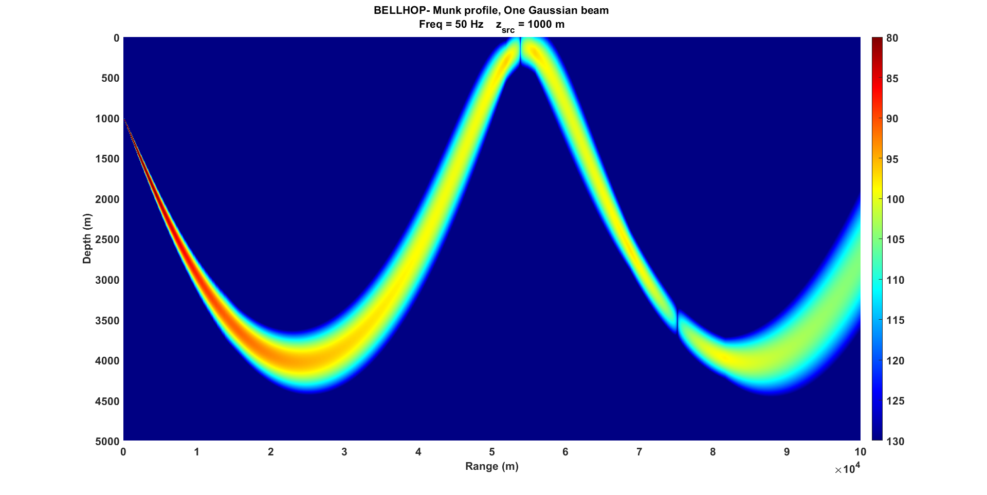
'Munk profile'        ! TITLE: Descriptive label for the simulation
50.0                  ! FREQ: Frequency in Hz
1                     ! NMEDIA: Number of media layers (usually 1 for ocean)
'CVW'                 ! SSPOPT: Sound speed interpolation type (e.g., C-linear, CVN, CVW)
51  0.0  20000.0      ! Number of SSP points, min and max depth
...                  ! Depth/sound speed profile follows
'A' 0.0               ! Altimetry model (usually flat surface)
20000.0  1600.00 0.0 1.8 0.8 /  ! Bathymetry: depth, speed, density, etc.

# Source coordinates
1                     ! NSx: number of source x positions
0.0 /                 ! x coordinate(s) in km
1                     ! NSy
0.0 /                 ! y coordinate(s) in km
1                     ! NSz
1000.0 /              ! Source depth in m

# Receiver grid
501                   ! NRz
0 5000 /              ! Receiver depths (0 to 5000 m)
1001                  ! NR
0.0  100.0 /          ! Receiver ranges (0 to 100 km)
2                     ! Ntheta
0.0 1.0 /             ! Receiver bearings (degrees)

# Run type (e.g., coherent, Gaussian beam, Nx2D)
'CG   3'              ! Option string: C=Coherent, G=Geometric beams, 3=3D mode

# Beam fans
51 6                  ! Nalpha, ISINGLE: Number of elevation beams and single-beam index
-14.66 14.66 /        ! Alpha (declination angles)
11 46                 ! Nbeta, ISINGLE: Number of azimuth beams and index
-2  2 /               ! Beta (bearing angles)

# Numerical integration
100.0  100.0 100.0 20500.0 ! STEP, Box%x, Box%y, Box%z (m, km, km, m)
Explanation of Bellhop3D Parameters
NSx,NSy,NSz: Number of source positions in x, y, and z.NRz,NR,Ntheta: Number of receiver positions in depth, range, and bearing.Alpha,Beta: Beam angles in elevation and azimuth.STEP: Integration step size.Box%{x,y,z}: Dimensions of the domain for ray propagation.OPTION(1:6): Specifies run type, beam type, directionality, source model, grid type, and dimensionality.
-
You can also download the sample notebook from here.
-
All code and setup files are also available on 📁 GitHub.
References
- Technical documentation: Ocean Acoustics Toolbox
- ARLPY Technical documentation: ARLPY Docs
- 📁 GitHub Repository (Code + Examples): Bellhop ARLPY ECED6575